Nicholas Day > Generating images with Flow Matching

2026-04-27

Flow matching

Top image generation models use flow matching (1). It can also be referenced as diffusion. Broadly, flow matching integrates a vector field ODE to generate an image, while diffusion integrates a SDE. There are many other formulations and perspectives on how diffusion/flow matching work. Recent work (2) shows that the flow matching framework allows for simpler constructions of the theory behind generation, subsuming diffusion as part of the framework. Flow matching allows for different losses and more direct paths from noise to image, so it trains faster and can achieve a higher quality, while also allowing for more efficient sampling.

To construct a flow matching model, first we start with a specific case. It's hard to sample directly from a complex data distribution, so we use continuous normalizing flows. These allow for iteratively transforming a simple distribution like Gaussians into a complex one like a sample of MNIST. A sequence of these distributions is called a probability path. In this case, we go from the Gaussian distribution to the Dirac Delta distribtion (deterministically returns one sample).

$$p_t(x|z) = N(\alpha_t z, \beta_t^2 I_d)$$

$p_t(x|z)$ samples from the distribution on this probability path at time $t$ with sample $z$ from the desired data distribution. At time $t=0$ , $\alpha_t = 0, \beta_t = 1$ . At time $t=1$ , $\alpha_t = 1, \beta_t=0$ . So this probability path progressively goes from no data, full noise to only the sample and no noise. These can be called noise schedulers in the literature.

With the flow matching formulation, we can choose an optimal transport noise schedulers (optimal transport is a theory that describes the optimal way to transport mass from one location to another). For this we choose:

$$\alpha_t = t \\ \beta_t = 1 - t$$

So when we sub in these noise schedulers, we get the Gaussian CondOT path. It flows linearly from the Gaussian to Dirac Delta distribution. Diffusion uses more complex noise schedulers that don't flow directly from initial to final distribution. A sample from this distribution at a point along the path would look like

$$x = zt + (1-t)\epsilon$$

In this equation, $x$ is the sample from the probability path, $t$ is a time from 0 to 1, $z$ is a sample from the data distribution, and $\epsilon$ is sampled Gaussian noise. It turns out that training on this Gaussian CondOT path works for sampling from the overall marginal distribution too (2)! So there's no complex and intractable integral that we need to evaluate.

To train on this distribution, we learn the flow matching vector field. The flow matching paper gives another result that the flow vector field at time t is

$$u_t(x|z) = (\dot{\alpha_t} - \frac{\dot{\beta_t}}{\beta_t}) z + \frac{\dot{\beta_t}}{\beta_t} x$$

When we plug in the Gaussian CondOT noise schedulers, this works out to be

$$u_t(x|z) = z - \epsilon$$

The final loss is then just

$$u_t^{\theta} - (z - \epsilon)$$

Architecture

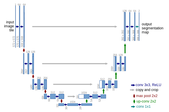
The original architectures used for diffusion models were U-Nets (3). They were invented in 2015 for medical image segmentation. They feature a series of bottlenecked convolutional stages with skip connections to allow for gradient flow.

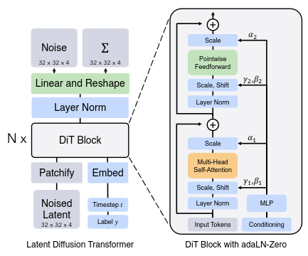
Most modern flow matching and diffusion implementations use diffusion transformers (DiT, 2022). They are based on vision transformers (ViT), which split images into square patches of pixel size p. Each patch is then embedded with a linear layer which matches the transformer token embedding size.

These image tokens then go through N DiT blocks which feature the adaptive layer norm. This is based on feature wise linear modulation (4) and adaptive instance normalization (5) which have shown to be effective conditioners used in GANs previously. The basic idea is to have an embedding which outputs scalars which either scale, shift, or modify the outputs / inputs of layers. This conditioning embedding's input is based on a sinusoidal positional embedding of the time (similar to original transformer paper), along with the input's class.

For MNIST, it's not necessary to train diffusion transformers on the latent of a VAE. But for most modern image generation, VAEs like the one used in Stable Diffusion are used.

Guidance

To generate images conditioned on a particular class, we use classifier free guidance. This section goes into a brief background on how it's derived.

The basic method of making a joint distribution on class label and images doesn't generate great quality samples empirically. Score based formulations of the loss were used to provide more emphasis on the label resulting in vector fields like

$$u_t(x|y) = u_t(x) + w a_t \nabla p_t(y|x)$$

However, this requires a classifier of noised data to predict a label. Ideally training two networks wouldn't be necessary, so classifier free guidance was derived as equivalent to the above vector field.

$$u_t(x|y) = (1-w) u_t(x) + w u_t(y|x)$$

In practice with 10 object classes that are being trained on, a null class is added to the list of categories to make 11 classes. While training with a given dropout probability, the labels are dropped and the model is trained with a null class.

During sampling, $u_t(x|y)$ is used with different guidance scales ($w$ as 1.0, 3.0, 5.0, etc) to improve adherence to prompts.

Discussion

There's a lot more to flow matching than in this post, this is just a brief overview. Other formulations and foundations worth looking into include the diffusion paper, score-based generative models, normalizing flows, and neural ODEs.

Some recent work like consistency models and mean flows show promising results for directly mapping noise to images with one neural net evaluation instead of 10s of iterations with ODE integration.

Diffusion has been applied with success to images, video, audio (review paper), and robotics ($\pi_0$ , diffusion policy), and animation (Diffuse-CLoC)

For more learning resources, check out MIT Flow Matching course, Bo Zhu's CGAI Diffusion assignment, and Mario Gemmoll Flow Matching Visualizer.