Nicholas Day > Optimizing fast and dynamic quadrotor trajectories

2026-08-25

A rendering of my quadrotor sim executing the optimized trajectory using a geometric controller.

One of the foundational pieces of quadcopter motion is making a quadcopter fly through waypoints relatively fast, so I wanted to give it a try in a custom simulator.

Simulator

I wrote the simulator from scratch because it's helpful for me to gain more understanding of how it works, along with practicing patience when it's utterly broken.

Luckily, the VNAV MIT Lectures have a great lecture on how to derive the force matrix which translates from rotor speeds to forces and torques, along with the basic dynamics model. However, quadrotors can't immediately go from 0 RPM to 39k RPM, so ideally there would be a model for that in the simulator too.

Originally I was going to model the 3 phase BLDC dynamics exactly, but then I remembered that I had the rest of the project to do too. So I chose to model it as a brushed DC motor. I believe this is approximately correct when using sensored field oriented control on the BLDC motors, but I know drones don't usually do this. A better approximation would be a good next step in the future. Here's the equation and code I ended up using:

$\dot{I} = (V_{a} - k_e * \omega - I_q * R) / L$

def sim(state, target):
    I_q = state[0]
    omega = state[1]

    cmd = 0.08 * (target - omega)

    target_voltage = k_e * target + cmd

    V_applied = min(target_voltage, Vsupply)

    I_dot = (V_applied - k_e * omega - I_q * R) / L
    omega_dot = (k_t * I_q) / J

    omega += omega_dot * dt
    I_q += I_dot * dt

    return [I_q, omega]

There's a small P-only loop in there with a feedforward too to ensure stable and fast RPM tracking. For the inertia (3 blade rotor and cylindrical motor shell) and Kv constants, I just used a 2207 drone racing motor and prop. Looks like a standard Kv for a 5 inch racing drone is about 1800Kv (RPM/V).

I did end up having some numerical integration issues with the motor sim and the sim broadly. The motor sim needs to run at ~10khz or it gives nonsense values. Probably relates to the time constant of the system. The outer sim itself I ran at 1khz. So every sim step, I'd run 10 motor loops. There were also a few fun bugs where things overflowed or underflowed when tuning the controller. It was common for my rotation matrix or omegas to get really large, blowing up the rest of the sim. I haven't fully debugged those yet, just changed tunable coefficients to be more reasonable.

The renderer uses C and Raylib. It just reads positions and orientations from a text file that the Python sim outputs and draws to the screen. I had a few (also very fun) bugs going from Z-up, X-forward (sim) to Z-forward, X-right (Raylib).

Geometric Control

At first, I had a very complicated set of cascaded PID loops. Going from position -> velocity -> angle -> motor RPM. That's easily 5-10 coefficients depending on how it's implemented. But it was such a pain to tune and wasn't even that performant because it relied on quasi-hover conditions, so it ended up shaking a lot.

Turns out that there's a geometric controller which computes the desired rotation angle by projecting the desired force vector onto what the quadrotor is capable of. Not only is it more performant, it has only 4 main constants to tune! So I ended up writing a simplified version based on this VNAV lecture. I also added integral control from this further follow up paper by the original authors to help with more stable tracking.

As far as tuning goes, I still had a hard time. But once I realized that the "inner" rotation loop should be tuned first (kR and kOmega) it was smooth sailing. I started with a target rotation with the position coefficients at zero, then graduated to the position terms when that seemed to track well. kP and kR can be thought of as "proportional" terms, with kV and kOmega as "damping" or velocity tracking terms. I generally tuned the kP and kR terms high with the kV and kOmega at about 20% of the position terms.

Trajectory Optimization

Before starting this project, I thought that trajectory optimization was this huge unapproachable topic, reserved for the ultra-committed. This paper by the founders of Skydio details how to model optimizing a multi segment trajectory through waypoints with constraints on the derivatives (i.e. initial vel / acc / jerk = 0 at start and end) using polynomial functions.

They show the equations for writing these constraints as linear (Ap = b) where p is the vector of coefficients of the segment's polynomial, and b are the derivative values choosen. Along with linear constraints that set the derivatives of the end of one trajectory equal to the start of the next trajectory.

This is then formulated into an objective J = \int (P^{(4)})^2 dt, which minimizes the snap derivative (4th) of the polynomial segments. J is easily solvable because it can be reformulated into a convex (quadratic) optimization problem by taking the Hessian (J = p^T Q P). These quadratic programs (QP) can be solved in under a millisecond!

However, with more than a few segments, this becomes numerically unstable. Some of the coefficients of these polynomials are really small and near the limit of computer precision. Luckily, the authors have a nice result for that too.

The linear constraints can be inverted to put J in terms of the derivative values.

$J = b^T A^{-T} Q A^{-1} b$

But, then the optimization is using all of the fixed derivatives (waypoints, acceleration / velocity constraints) and free-to-optimize derivatives as optimization variables. A permutation matrix can be formulated that partitions the vectors into fixed, then free. This allows for separating the J matrix into blocks of fixed and free portions, resulting in this expression, with F being fixed, and P being the derivatives we want to optimize over.

$J = b_F^T R_{FF} b_F + b_F^T R_{FP} b_p + b_p^T R_{PF} b_F + b_p^T R_{pp} b_p$

This was confusing and daunting for me at first, but all of the R are constants. R is also symmetric so R_{FP} and R_{PF} are symmetric. J is now of the form:

$J = p^T Q p + c^T p$

Now that we have an unconstrained quadratic program, this can be reduced to taking the derivative and setting it equal to zero, then solving for x (Boyd, pg 457). Just like in single variable calculus!

The optimal derivatives for multi segment trajectory optimization are then

$b_P = -R_{PP}^{-1} R_{FP}^T b_F$

To solve for the polynomial coefficients, b_P is mixed with b_F using the permutation matrix and multiplied by the block diagonal matrix A^{-1} which encodes the constraints for derivatives equal between segments and specified derivatives.

$Ap = b \\ p = A^{-1} b$

After finally integrating all of these parts together, I did have a few integration hell type bugs.

My first big bug was that I had read in an earlier paper (Mellinger and Kumar, a classic) that they used a similar approach and time scaled the polynomial after trajectory generation. However, I had forgotten to multiply by the time scaling factor due to chain rule. This resulted in huge velocities that my quadrotor couldn't meet because the trajectory expected every segment to last 1 second.

My second big bug was that the quadrotor's Z wasn't tracking well.

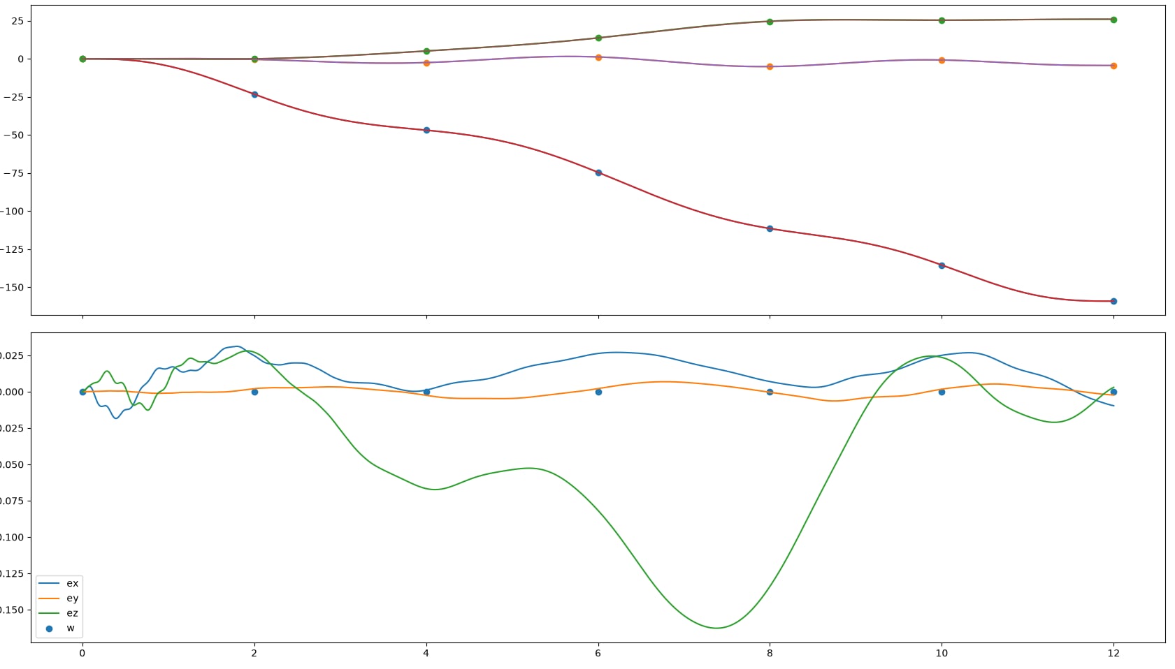
Top is the expected vs actual trajectory, bottom is the error. The Z was off by ~6 inches at the worst. Turns out for the feedforward acceleration term, I was using the velocity derivative for the Z component. I learned this after I implemented integral control on top of the existing geometric control to fix this...

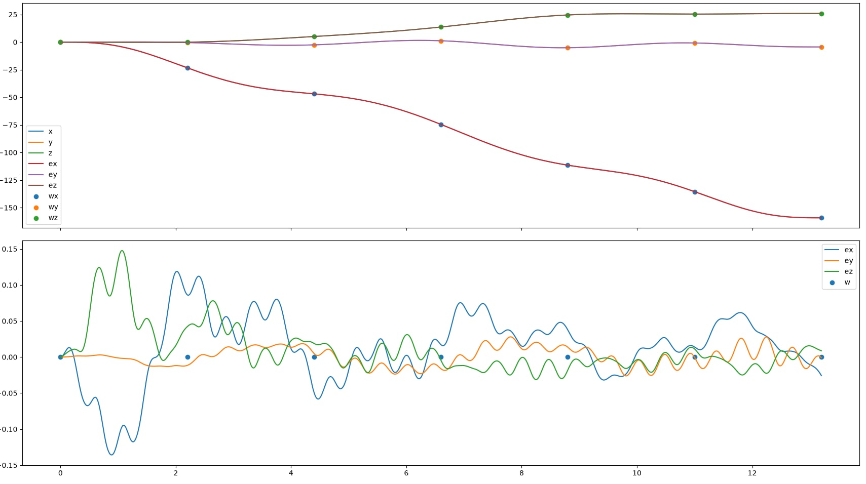
Now all trajectories match to waypoints within about an inch, pretty nice.

Future work

There are a few bugs left in this system. Yaw control doesn't track very accurately (should be 0 degrees throughout the whole flight). I also didn't implement desired angular acceleration in the geometric controller. I expected it would help a lot, as desired acceleration was a big boost in accuracy too.

Bry et al used their QP optimization as an inner loop, with a probabilistic road map selecting waypoints that weren't intersecting obstacles. Dynamic obstacles and waypoints would be a good add.

They also had gradient descent in the outer loop to select the optimal time for each segment. This is pretty cool because it not only scales the times for the segments, but also makes harder segments slow down, and easier segments speed up. I just manually selected segment times that worked well enough.

It would be great to run this on a real robot, but for good position estimation there has to be either motion capture or vision-inertial based SLAM available, which I'm also working on from scratch. Stay tuned!

More modern papers can incorporate obstacle avoidance directly into the optimization (paper) using a simplified convex relaxation which is still relatively good. Trajectories can also be solved even faster with new formulations of the QP (paper). There are new controllers which are able to handle poorly modeled dynamics and disturbances well (INDI paper). Not to mention MPC and RL/DL based approaches.